Grid Physics from Scratch with pandapower

A lot of the security labs I came across while planning this skip the industrial part. They stand up a fake controller that returns canned numbers, and the dramatic “attack” at the end flips one of those numbers from a 0 to a 1. Nothing downstream cares, because there is no downstream.

So this post builds the electricity first. I use pandapower, a Python library that does the actual electrical math, to run a live simulation of a small power grid that computes the real voltages and currents at every point, the way the physical grid would. When you open a circuit breaker in it, the effects spread out: power reroutes down other lines, voltages sag, and some of those other lines start carrying more than they should. That’s the difference between a demo and a real model, and it’s what makes the attack three posts from now actually mean something.

A note on vocabulary, since this is where the industrial terms start. OT (Operational Technology) is the computing that touches physical equipment — as opposed to IT, which touches data. SCADA (Supervisory Control and Data Acquisition) is the control-room software an operator watches: it continuously polls field equipment for readings and sends commands back. And a bus, in power engineering, is not a data bus — it’s a physical node in the network, a point where lines, generators, and loads connect. When I say the simulation “solves bus voltages,” I mean it computes the voltage at each of those junctions.

There’s no security in this post yet, just physics that behaves like a real grid.

Where this fits. This is post 2 of the series. It builds directly on the architecture from Why I Built a Fake Power Grid to Learn NERC CIP.

What is pandapower?

pandapower is a Python library that solves a real power flow — the numerical problem of figuring out, given a network of buses, lines, loads, and generators, what the voltage is at every bus and how much power flows on every line. It’s Python-native, pip-installable, and scriptable, which is exactly what I want: I can loop it on a timer and expose its results to the outside world programmatically.

The alternative I considered was OpenDSS (EPRI), which is better if you want feeder-level distribution modeling with quasi-static time series. I went with pandapower because I’m modeling a transmission-level control center, and pandapower ships recognizable transmission test cases out of the box.

Why I used real physics instead of fake numbers

I could have faked the numbers with a random-number generator, but that would defeat the whole point. When I later send an unauthorized breaker-open command over DNP3 (post 3), I want the grid to actually react: flows redistribute, voltages shift, lines get closer to their limits. If I’m really computing the physics, a scary-looking command turns into a measurable physical consequence, and that’s what gives the CIP-015 detection in post 5 something real to catch.

Setting it up

1. Spin up the OT-zone VM and install pandapower. This lives on a VM inside the ESP (the OT zone), not on the management side.

   python3 -m venv venv && source venv/bin/activate
   pip install pandapower
   

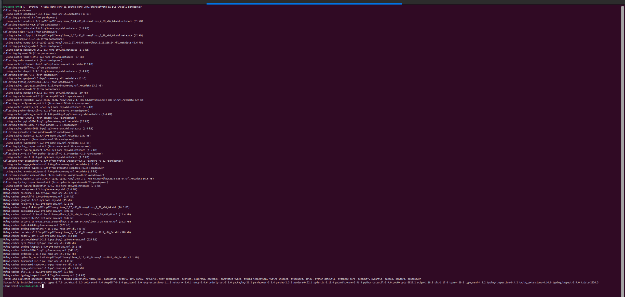   pandapower 3.5.4 installs clean, and brings about thirty transitive dependencies with it — numpy, scipy, pandas, networkx, pydantic. Worth noticing now: that’s the software inventory CIP-010 will ask me to baseline in post 6, and every one of those wheels came from the internet onto a machine that is supposed to live inside the perimeter.

   The first thing the ESP costs you. The OT zone is an isolated libvirt network — no NAT, no default route — so pip install cannot reach the internet, which is the entire point of building it that way. I gave the VM a second, temporary NIC on the NAT network, installed, then detached it and confirmed ping 8.8.8.8 fails again. That’s the real workflow in an OT environment: patching is a deliberate, logged, time-boxed event, not something a machine inside the perimeter does whenever it feels like it. Post 6 comes back to this as CIP-007 patch management.

2. Load a recognizable transmission case. I’m using case39, the IEEE 39-bus “New England” system — a case anyone in the field will recognize.

   import pandapower as pp
   import pandapower.networks as nw
   
   net = nw.case39()   # IEEE 39-bus "New England" transmission case
   

   Built-in cases worth knowing: case9(), case14(), case_ieee30(), case39(). Start small if you’re debugging; case39 is the one I’ll screenshot.

3. Solve the power flow and read the results. runpp runs the solver; the answers land in the net.res_* tables.

   pp.runpp(net)                          # solve the power flow
   print(net.res_bus.vm_pu.head())        # bus voltages (per unit)
   print(net.res_line.p_from_mw.head())   # line flows (MW)
   

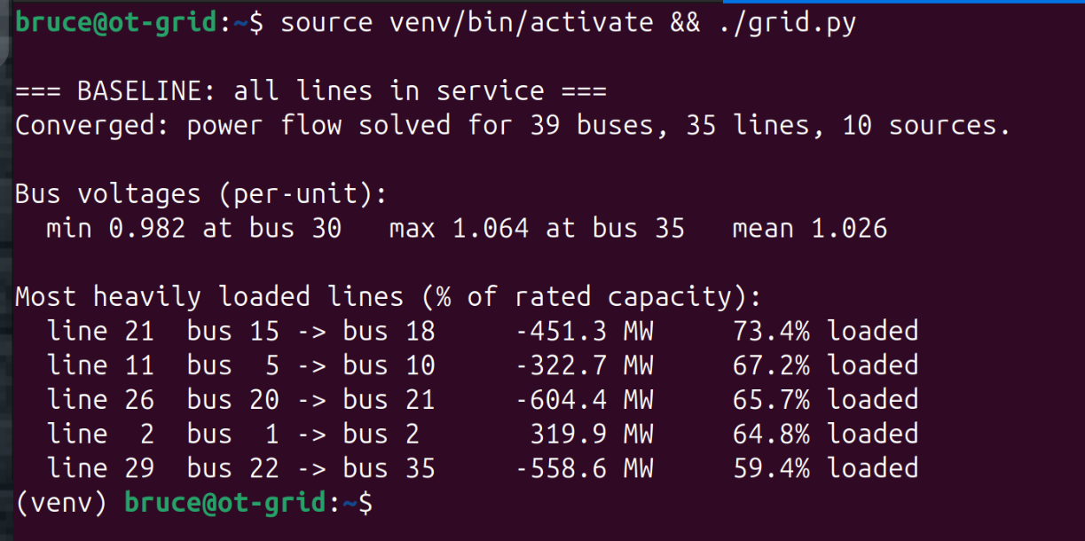   The solver converges: 39 buses, 35 lines, 10 sources. Voltages sit in a believable band (0.982–1.064 per unit), and the busiest circuit is line 21 at 73.4% of its rating. These are the analog values a SCADA master will poll over DNP3 in the next post — line 11’s 67.2% shows up again there, and in the chart below.

Making the grid update on a loop

A single solve is just a snapshot. A real grid changes all the time, so I run runpp on a loop and republish the results every cycle. That way the protocol layer always has fresh values to read.

while True:
    pp.runpp(net, numba=False)
    snap = snapshot(net)                 # bus voltages, line flows, breaker states
    STATE_PATH.write_text(json.dumps(snap, indent=2))
    time.sleep(2)

That snapshot is published two ways: to a JSON file on disk, and over HTTP on port 8080 — GET /state returns the current solve, POST /breaker takes a line out of service. Breaker commands land in the model and the next solve picks them up:

$ curl -s http://10.10.20.10:8080/state | jq '.analog.line_loading_pct["9"]'
38.06
$ curl -s -X POST http://10.10.20.10:8080/breaker -d '{"line": 12, "closed": false}'
{"line": 12, "closed": false}
$ curl -s http://10.10.20.10:8080/state | jq '.analog.line_loading_pct["9"]'
60.6

One HTTP POST, and line 9 jumps 22 points closer to its rating. That round trip, from a command to a new set of readings, is the link between the physics and the protocol layer. In the next post, OpenPLC (the DNP3 outstation) reads those analog values from a different VM and maps them to DNP3 points, and breaker commands come back the other way as a CROB instead of a curl. The effect on the grid is exactly the same, which is the whole point.

flowchart LR
    subgraph loop["Timed loop (every ~2s)"]
        solve["pp.runpp(net)"] --> res["net.res_bus / net.res_line<br/>net.line.in_service"]
        res --> pub["snapshot() →<br/>JSON file + HTTP :8080"]
    end
    pub -->|"analog values up"| proto["Protocol layer<br/>(DNP3 outstation — post 3)"]
    proto -->|"breaker command down"| solve

Build note — this bites you later if you skip it. Put pandapower and the DNP3 outstation on separate VMs inside the ESP. If they talk over localhost on one host, the protocol traffic never crosses a monitored segment and the CIP-015 sensor in post 5 sees nothing. Make the physics and the protocol talk over the wire on purpose.

Verifying it worked

The grid is behaving if two things are true: the solve converges every cycle, and toggling a breaker changes the flows. A quick check — open a line and confirm power redistributes:

net.line.at[12, "in_service"] = False   # "open a breaker" on line 12 (bus 6 <-> bus 7)
pp.runpp(net, numba=False)
print(net.res_line.loading_percent)     # flows should differ from the closed-breaker solve

They do, and the change is big. The power that was crossing bus 6 → bus 7 has to get there some other way, so it piles onto the neighbouring lines:

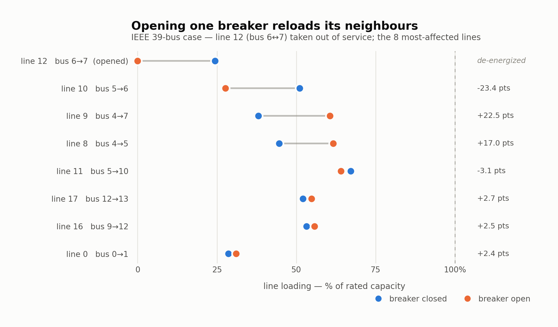
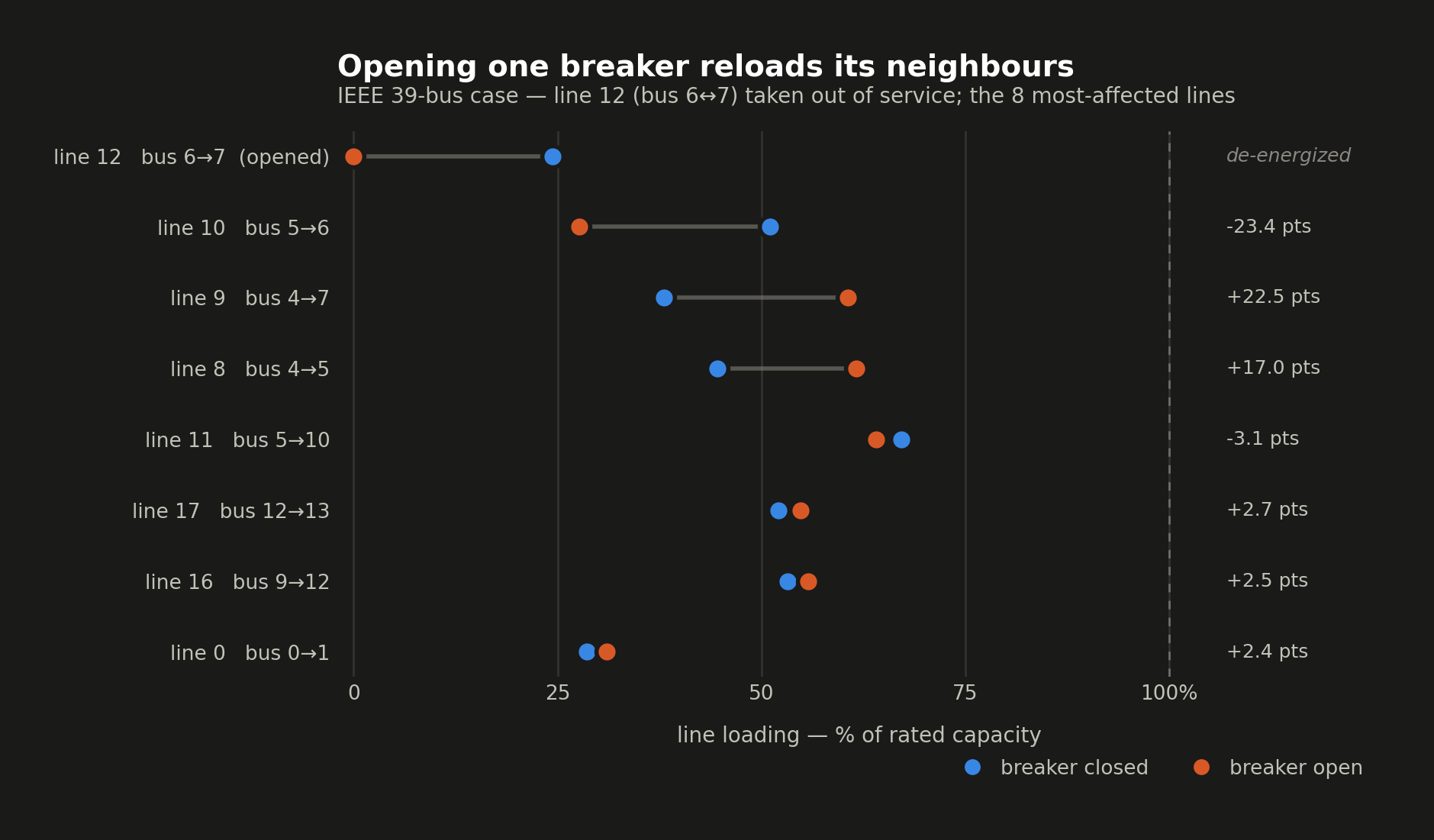Line 12 goes to zero. Lines 9 and 8 each end up roughly 20 points closer to their rated capacity than they were a second earlier — and line 10 sheds 23 points, which is the most interesting number on the chart.

Nothing told line 9 to pick up 22 points of load; that’s just Kirchhoff’s laws playing out. If you open enough of the right breakers, one of those neighbouring lines goes past 100%, and then its own protection relay trips it out too and pushes its load onto the next line along. That’s how a cascading outage happens, and it’s why a single unauthorized command here is a physical event, not just a lost data point.

But look again at line 10, because it goes the other way: −23.4 points, the biggest single change on the chart apart from the breaker I actually opened. It’s worth explaining, because it’s where the simple “load spills onto the neighbours” picture stops holding.

Bus 6 has a 233.8 MW load of its own. Bus 7, on the far side of the breaker, has 522 MW. With everything closed, line 10 was carrying 453.8 MW into bus 6 — enough to serve bus 6, with 218.8 MW left over to continue through line 12 to bus 7. Line 10 wasn’t just feeding bus 6; it was a transit path to bus 7.

Open line 12 and that transit job disappears. Line 10 settles at 234.2 MW — almost exactly bus 6’s own load, and nothing more. Bus 7’s missing supply doesn’t vanish; it comes the long way round instead, and you can watch it arrive: line 9 gains 204 MW, fed by the same 204 MW increase on line 8. The power is conserved, the route just changed, and line 10 got quieter because it stopped being a through-path.

This matters more than it looks. If you built an alarm that only watched for circuits getting hotter, it would have caught lines 9 and 8 and completely missed the biggest change in the system. Real control rooms run state estimation and contingency analysis across the whole network for this reason, and the same trap shows up again in post 5: an attack doesn’t reliably look like “a number went up.”

Pros and cons

Pros	Cons
Real solver → real physical consequences to detect later	Not a real-time simulator; the timed loop is an approximation
Python-native, scriptable, trivial to expose to a protocol layer	Transmission-level; no feeder detail (use OpenDSS if you need that)
Recognizable IEEE test cases lend credibility	You own the seam between physics and protocol — extra plumbing

Wrap-up

At this point I have a working grid simulation: it solves continuously, exposes its analog values, and reacts when I open or close a breaker. It’s still completely unprotected and doesn’t speak any OT protocol yet. In the next post I put it on the wire with OpenPLC as a DNP3 outstation, which is where the attack surface becomes real.

References

• pandapower · repo · docs
• OpenDSS (EPRI) — distribution-level alternative
• OpenPLC Runtime (Autonomy-Logic) — the DNP3 outstation, next post
• NERC Reliability Standards (United States)